

Building an amortization schedule in Excel is one of the most fundamental tasks in financial modeling, and one of the most commonly done wrong. Most people build their schedule in a separate tab, fill it with correct-looking numbers, and then manually copy figures into their income statement, cash flow statement, and balance sheet. That works until an input changes. Adjust the loan amount, the interest rate, or the term, and suddenly three parts of the model are out of sync, turning the schedule into a liability instead of a tool.
A properly constructed amortization schedule does more than list payments. It splits every payment into interest and principal, tracks the declining balance period by period, and feeds directly into the financial statements through live formula links. When the loan inputs change, the entire model updates. That is the standard worth building toward, and this guide covers every layer to get you there.
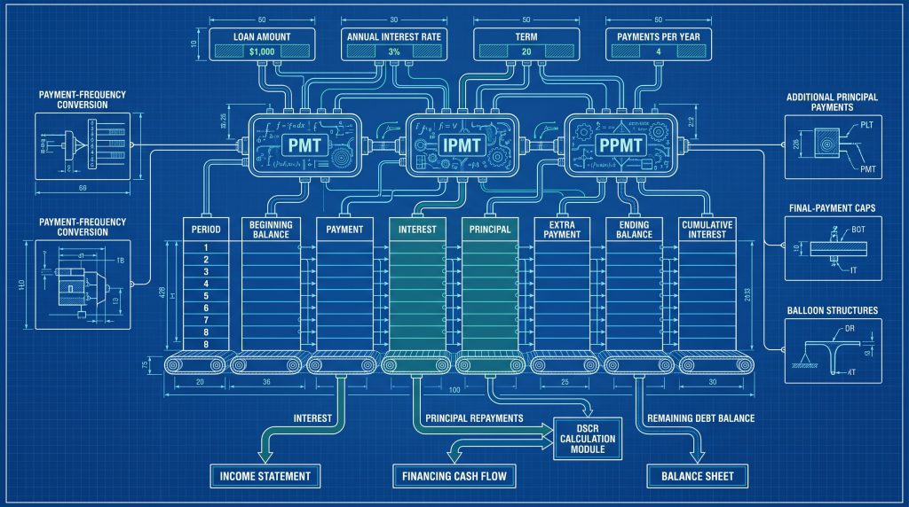
You will find the full build sequence here: from the four inputs your schedule cannot function without, through PMT, IPMT, and PPMT formulas, to extra payments, balloon structures, and multi-frequency schedules. For those who want this architecture already assembled and linked to a full three-statement model, Best Financial Models (BFM) can provide a loan repayment model template built to that specification. But first, understand what you are building and why each decision matters.

Amortization works on a simple principle: interest for each period is calculated on the outstanding balance at the start of that period. Early in the loan, the balance is high, so a large portion of each payment goes to interest and only a small slice reduces the principal. As the balance falls, less interest accrues, and more of each fixed payment chips away at what you actually owe. The payment amount never changes; its composition does, shifting gradually from interest-heavy to principal-heavy across the life of the loan.
This shift is not intuitive until you see it row by row in a table. Borrowers who have never looked at a schedule often assume they are paying down their loan at a steady rate from day one. The schedule corrects that assumption immediately and makes the real cost of debt visible.
Take a $200,000 loan at 7% over 20 years. The monthly payment comes to roughly $1,551. In the first month, interest on the full $200,000 balance at a 7% annual rate equals approximately $1,167. That means only $384 of that first payment actually reduces the principal. After twelve months of payments, you have paid over $18,600 but reduced the balance by less than $5,000. The schedule makes this concrete, which is why lenders and investors commonly expect to see it modeled correctly.
Over the full 20-year term of that same $200,000 loan, the borrower pays roughly $172,000 in total interest, nearly the original loan amount again. That figure is invisible if you only look at the monthly payment. The amortization schedule surfaces it in the final row of a cumulative interest column, and for any investor or lender reviewing a funding application, that number directly affects how they assess the project’s debt carrying capacity and free cash flow.
Every functional amortization schedule runs on four inputs: the loan amount (the present value), the annual interest rate, the loan term in years, and the payment frequency. These belong in clearly labeled, individually referenced cells at the top of your worksheet, not hardcoded inside formulas. When these inputs sit in dedicated cells, changing any one of them recalculates the entire schedule automatically. That is what separates a dynamic model from a static table.
Excel’s named range feature lets you assign a readable label to any cell. Instead of referencing $B$2 buried inside a 60-character formula string, you reference AnnualRate. The formula reads like a sentence, and anyone opening the file- an auditor, a lender, or a colleague- can follow the logic without a walkthrough. To define a name, select the cell, click in the Name Box to the left of the formula bar, and type your label. Apply the same approach to LoanAmount, TermYears, and PaymentsPerYear . Microsoft’s Excel documentation covers named ranges in detail if you need a UI reference.
This is where more amortization schedules go wrong than anywhere else. Every Excel finance function assumes the rate and the period count are in the same unit. For a monthly schedule, you divide the annual rate by 12. For a biweekly schedule, you divide by 26. For a weekly schedule, you divide by 52. If you build your schedule with a PaymentsPerYear input cell, you never have to hardcode this conversion; every formula in the table references the same input, and switching frequencies requires only one cell change.

The PMT function calculates the constant payment amount for a loan given a fixed rate, number of periods, and present value. The syntax for a monthly schedule is: =PMT(AnnualRate/12, TermYears*12, -LoanAmount). The loan amount is entered as a negative because it represents a cash outflow from the lender’s perspective, money leaving the bank and coming to you. PMT returns the payment as a positive number when the present value is negative, which keeps your schedule readable without sign-convention confusion.
IPMT calculates the interest portion of a specific period’s payment: =IPMT(AnnualRate/12, PeriodNumber, TermYears*12, -LoanAmount). PPMT calculates the principal portion for that same period: =PPMT(AnnualRate/12, PeriodNumber, TermYears*12, -LoanAmount). Both functions require the period number as an argument, which is why the period column in your schedule must increment correctly from row to row. The relationship to verify before building the full table: IPMT + PPMT should equal PMT for every period on a standard level-payment loan where payments fall at period end. If the result does not match, check your rate conversion, period references, and the optional type argument, setting type to 1 (payments at the beginning of the period) changes the calculation and can break this relationship if applied inconsistently.
Before dragging formulas across 120 or 240 rows, run this verification. Multiply your PMT result by the total number of payments to get gross cash outflow. Subtract the original loan amount. The remainder should equal your total interest cost. Now calculate total interest independently: sum the IPMT results for all periods (you can use a quick SUMPRODUCT for this). If both figures match, your inputs and formulas are correctly wired. If they diverge by even a cent, find the error before it propagates through every row of the schedule.
A clean, functional amortization table uses eight columns: Period, Beginning Balance, Payment, Interest, Principal, Extra Payment, Ending Balance, and Cumulative Interest. Separating beginning and ending balance is a deliberate structural choice. It forces each row to reference the prior row’s ending balance as its starting point, creating a chain of dependent calculations that gives the table its dynamic character. If you skip this separation and calculate balance from scratch in each row, you lose the ability to model extra payments or accelerated payoff correctly.
Row one is the foundation. The Beginning Balance cell references your LoanAmount input directly. Payment uses the PMT formula with absolute references to all input cells so it does not drift when copied down. Interest uses IPMT with the period number as a relative reference (so it increments each row) and the input cells as absolute references. Principal uses PPMT in the same structure. Ending Balance equals Beginning Balance minus the Principal value. Lock down the formulas in this first row before extending them, because every subsequent row inherits this logic.
With absolute references on all input cells and a relative reference on the period number, every formula updates correctly when you fill down through the full term. One sign-convention issue comes up consistently: PPMT returns a negative value by default, which can make the Ending Balance formula produce unexpected results. The clean fix is to wrap the PPMT reference in a negative sign: =BeginningBalance, (-PPMT(...)), or equivalently, structure your ending balance as =BeginningBalance + PPMT(...) since PPMT is already negative. Decide on your convention in row one and apply it consistently throughout.
For users on Excel 365 or Excel 2021, the SEQUENCE function eliminates manual period numbering entirely. =SEQUENCE(TermYears*12) generates the full period column as a single spilled array. Pair this with array-enabled IPMT and PPMT formulas and the entire table populates from a single formula block. The real advantage appears when the term input changes: SEQUENCE automatically adjusts the number of rows, so a 10-year schedule does not leave 60 empty rows with broken formula references at the bottom of a 5-year term. For earlier Excel versions, fill down manually after locking the input references.
The structural change is minimal, but the impact on model accuracy is significant. Insert a column labeled Extra Payment between the Scheduled Principal column and the Ending Balance column. Users enter additional principal payments directly into specific cells in this column, a one-time lump sum in the period it occurs, or a recurring amount copied down through every row. The Payment, Interest, and IPMT formulas remain completely untouched. Only the Ending Balance formula changes to account for the additional reduction in principal.
The revised ending balance formula subtracts both the scheduled principal and the extra payment from the beginning balance: =BeginningBalance, ScheduledPrincipal, ExtraPayment. Because extra payments reduce the outstanding balance immediately, every subsequent row inherits a lower starting balance, which reduces the interest charge in those periods and in turn accelerates the principal reduction. The effect compounds across the remaining term, shortening the loan payoff date and reducing total interest. This is what makes the extra payment column analytically useful rather than decorative.
The edge case that breaks a clean schedule is an extra payment that exceeds the remaining balance in the final period. Without a cap, your ending balance formula produces a negative number, the loan technically ends mid-row, and the schedule keeps calculating interest on a negative balance. Cap the extra payment so it never exceeds the remaining balance after the scheduled principal is applied: =MIN(ExtraPaymentInput, BeginningBalance, ScheduledPrincipal). This ensures the extra payment draws the balance to zero at most, so the schedule ends cleanly in the correct period. Once the beginning balance reaches zero, the formula naturally returns zero as well, no additional IF logic required for standard loan structures.
Instead of hardcoding 12 in every rate-conversion and period-count formula, add a single input cell labeled PaymentsPerYear. Reference this cell in the PMT rate argument (AnnualRate/PaymentsPerYear) and in the period count (TermYears*PaymentsPerYear). With this structure in place, switching from monthly to biweekly to weekly requires changing exactly one cell. No formula rewriting, no risk of updating some occurrences and missing others.
Two different approaches carry the label “biweekly,” and they produce meaningfully different results. The strict actuarial method sets PaymentsPerYear to 26 and calculates PMT directly on that basis: =PMT(AnnualRate/26, TermYears*26, -LoanAmount). This spreads the annual obligation across 26 payments but does not inherently accelerate payoff; the borrower is simply paying on a tighter schedule, not making additional principal payments. The accelerated biweekly convention, which many mortgage lenders market as a payoff-shortening product, calculates the standard monthly PMT and divides it by two. Because 26 half-monthly payments equal 13 full monthly payments per year, this approach effectively adds one extra monthly payment annually and does shorten the loan term.
Use the strict 26-period method when your loan contract amortizes on a 26-payment-per-year basis. Use the half-monthly convention when your lender specifically markets an accelerated biweekly product. The difference in total interest over a 20-year loan can be material, so matching the method to the contract matters for accurate debt service projections.
For a $200,000 loan at 7%, the difference in total interest between monthly and strict 26-period biweekly amortization is modest, since both methods cover the same annual obligation. The accelerated biweekly convention, where the borrower makes the equivalent of 13 monthly payments per year, can meaningfully shorten the effective payoff date and reduce cumulative interest. For project finance models where a lender is stress-testing DSCR across a 15-year loan term, the payment frequency assumption directly affects every year’s debt service calculation and every covenant test. Use the method that matches the loan contract, not the one that looks best in the model.
A balloon loan structures regular periodic payments to cover interest plus a limited amount of principal, leaving a large residual balance that comes due in a lump sum at maturity. These structures appear frequently in commercial real estate, development finance, and infrastructure project loans, where the borrower expects to refinance or sell the asset before the balloon date. In the amortization table, every row prior to the maturity date looks like a normal partial-amortization schedule. The final row carries an additional column for the balloon payment, which equals whatever outstanding balance remains after the last scheduled payment.
The table modification is straightforward. Add a column labeled Balloon Payment. In all rows except the final one, this column is zero. In the maturity row, the cell contains the outstanding beginning balance for that period, either entered directly or pulled from the prior row’s ending balance formula. Update the Ending Balance formula in the final row to net to zero: =BeginningBalance + Interest, ScheduledPrincipal, BalloonPayment. For interest-only balloon structures, remove PPMT from the periodic rows entirely and replace it with a simple =BeginningBalance * PeriodicRate calculation, since no principal amortizes until the balloon date.
Banks and development finance institutions frequently align balloon maturities with project milestones, an asset completion date, a refinancing event, or a planned equity exit. A financial model that handles balloon payments correctly shows lenders exactly what the debt service looks like in every period and what the terminal cash requirement is at maturity. This supports accurate DSCR calculations through the loan term and gives equity investors a clear picture of the refinancing risk embedded in the capital structure. A model that ignores the balloon and shows zero balance in the final period misstates both cash flow and risk significantly.
The interest column in the amortization schedule is the direct source for interest expense on the income statement. In a properly integrated three-statement model, the debt schedule feeds period-by-period interest to the income statement through a formula link rather than a flat percentage estimate. This matters because interest expense changes over time as the loan balance declines. A flat estimate overstates interest in later periods, overstates costs, understates net income, and produces an incorrect tax calculation. The amortization schedule eliminates all of that by supplying the exact figure for each period.
Principal repayments do not appear on the income statement. They reduce the long-term debt liability on the balance sheet and flow through the financing activities section of the cash flow statement. This distinction is one of the most persistent errors in poorly built three-statement models. A modeler routes the full loan payment through the income statement, treats principal as an expense, and the balance sheet no longer balances. The amortization schedule makes the separation clean: the interest column feeds operating expenses, and the principal column feeds both the financing cash flow and the balance sheet debt balance through separate formula links with no overlap.
Debt Service Coverage Ratio equals net operating income divided by total debt service for a given period. Total debt service is the sum of interest and principal repayments, which your amortization schedule provides directly. The formula in Excel is: =NOI_Cell / (InterestColumn + PrincipalColumn) for each period, or using annual totals for a yearly DSCR output. Lenders set minimum DSCR covenants, often 1.20x or 1.25x for commercial real estate, and they test compliance in every year of the loan term. A model with a correctly structured amortization schedule gives a reliable, formula-driven DSCR output that updates automatically when revenue assumptions or loan terms change.
An amortization schedule answers one specific question: how does this loan repay over time? A financial model uses that schedule as one input among many, integrating debt service with revenue projections, operating costs, capital expenditure, working capital movements, and tax assumptions to produce a complete picture of business performance. The schedule without the model is like a building’s structural drawing without the architectural plans. Building the connection between them is what separates a financial analyst’s output from a basic spreadsheet.
The build sequence for a complete amortization schedule in Excel follows a clear order. Start with the four input cells and name them for readability. Calculate your periodic rate conversion and confirm it before writing any table formulas. Use PMT to lock in the payment, then IPMT and PPMT to populate the interest and principal columns, with absolute references on all inputs and a relative reference on the period number. Run the sense check before filling down. Add the extra payment column and update the ending balance formula. Layer in the balloon column if the loan structure requires it. Add the PaymentsPerYear input to make the frequency switchable without rewriting any logic.
Every one of those steps is valuable, but the schedule only reaches its full potential when it connects to the rest of a financial model. Interest expense links to the income statement. Principal feeds the balance sheet and financing cash flows. DSCR calculates from live formula references. That integration is what lenders and investors need to see, and it is what separates a professional financial model from a well-formatted spreadsheet.
If you want that integration ready from the start, the BFM loan repayment model template provides a structured, fully wired starting point already linked to complete financial statements. Download it, enter your loan parameters, and you have a bank-ready debt schedule in minutes rather than hours. Or build your own from scratch using the formulas in this guide. Either way, the goal is the same: a dynamic, connected amortization schedule in Excel that gives you and your stakeholders an accurate, auditable picture of every dollar of debt service across the full loan term.
If you are looking for assistance in writing a funder-ready business plan, then contact JTB Consulting for further assistance. They have written thousands of bankable business plans since their establishment in 2006.